Quick Start Tutorial#
GluonTS contains:
A number of pre-built models
Components for building new models (likelihoods, feature processing pipelines, calendar features etc.)
Data loading and processing
Plotting and evaluation facilities
Artificial and real datasets (only external datasets with blessed license)
[1]:
# %#matplotlib inline
import mxnet as mx
from mxnet import gluon
import numpy as np
import pandas as pd
import matplotlib.pyplot as plt
import json
Datasets#
Provided datasets#
GluonTS comes with a number of publicly available datasets.
[2]:
from gluonts.dataset.repository.datasets import get_dataset, dataset_recipes
from gluonts.dataset.util import to_pandas
[3]:
print(f"Available datasets: {list(dataset_recipes.keys())}")
Available datasets: ['constant', 'exchange_rate', 'solar-energy', 'electricity', 'traffic', 'exchange_rate_nips', 'electricity_nips', 'traffic_nips', 'solar_nips', 'wiki-rolling_nips', 'taxi_30min', 'kaggle_web_traffic_with_missing', 'kaggle_web_traffic_without_missing', 'kaggle_web_traffic_weekly', 'm1_yearly', 'm1_quarterly', 'm1_monthly', 'nn5_daily_with_missing', 'nn5_daily_without_missing', 'nn5_weekly', 'tourism_monthly', 'tourism_quarterly', 'tourism_yearly', 'cif_2016', 'london_smart_meters_without_missing', 'wind_farms_without_missing', 'car_parts_without_missing', 'dominick', 'fred_md', 'pedestrian_counts', 'hospital', 'covid_deaths', 'kdd_cup_2018_without_missing', 'weather', 'm3_monthly', 'm3_quarterly', 'm3_yearly', 'm3_other', 'm4_hourly', 'm4_daily', 'm4_weekly', 'm4_monthly', 'm4_quarterly', 'm4_yearly', 'm5', 'uber_tlc_daily', 'uber_tlc_hourly', 'airpassengers']
To download one of the built-in datasets, simply call get_dataset with one of the above names. GluonTS can re-use the saved dataset so that it does not need to be downloaded again the next time around.
[4]:
dataset = get_dataset("m4_hourly")
In general, the datasets provided by GluonTS are objects that consists of three main members:
dataset.trainis an iterable collection of data entries used for training. Each entry corresponds to one time series.dataset.testis an iterable collection of data entries used for inference. The test dataset is an extended version of the train dataset that contains a window in the end of each time series that was not seen during training. This window has length equal to the recommended prediction length.dataset.metadatacontains metadata of the dataset such as the frequency of the time series, a recommended prediction horizon, associated features, etc.
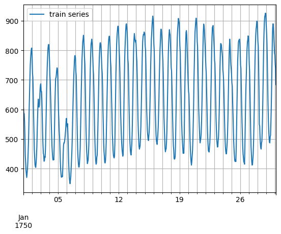
[5]:
entry = next(iter(dataset.train))
train_series = to_pandas(entry)
train_series.plot()
plt.grid(which="both")
plt.legend(["train series"], loc="upper left")
plt.show()
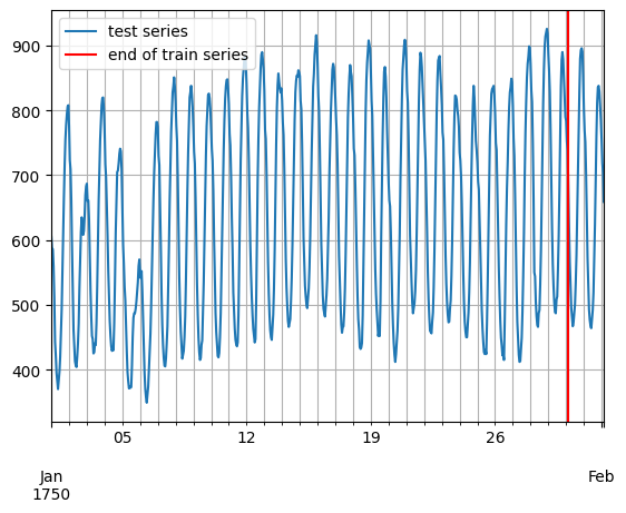
[6]:
entry = next(iter(dataset.test))
test_series = to_pandas(entry)
test_series.plot()
plt.axvline(train_series.index[-1], color="r")  # end of train dataset
plt.grid(which="both")
plt.legend(["test series", "end of train series"], loc="upper left")
plt.show()
[7]:
print(
    f"Length of forecasting window in test dataset: {len(test_series) - len(train_series)}"
)
print(f"Recommended prediction horizon: {dataset.metadata.prediction_length}")
print(f"Frequency of the time series: {dataset.metadata.freq}")
Length of forecasting window in test dataset: 48
Recommended prediction horizon: 48
Frequency of the time series: H
Custom datasets#
At this point, it is important to emphasize that GluonTS does not require this specific format for a custom dataset that a user may have. The only requirements for a custom dataset are to be iterable and have a “target” and a “start” field. To make this more clear, assume the common case where a dataset is in the form of a numpy.array and the index of the time series in a pandas.Period (possibly different for each time series):
[8]:
N = 10  # number of time series
T = 100  # number of timesteps
prediction_length = 24
freq = "1H"
custom_dataset = np.random.normal(size=(N, T))
start = pd.Period("01-01-2019", freq=freq)  # can be different for each time series
Now, you can split your dataset and bring it in a GluonTS appropriate format with just two lines of code:
[9]:
from gluonts.dataset.common import ListDataset
[10]:
# train dataset: cut the last window of length "prediction_length", add "target" and "start" fields
train_ds = ListDataset(
    [{"target": x, "start": start} for x in custom_dataset[:, :-prediction_length]],
    freq=freq,
)
# test dataset: use the whole dataset, add "target" and "start" fields
test_ds = ListDataset(
    [{"target": x, "start": start} for x in custom_dataset], freq=freq
)
Training an existing model (Estimator)#
GluonTS comes with a number of pre-built models. All the user needs to do is configure some hyperparameters. The existing models focus on (but are not limited to) probabilistic forecasting. Probabilistic forecasts are predictions in the form of a probability distribution, rather than simply a single point estimate.
We will begin with GluonTS’s pre-built feedforward neural network estimator, a simple but powerful forecasting model. We will use this model to demonstrate the process of training a model, producing forecasts, and evaluating the results.
GluonTS’s built-in feedforward neural network (SimpleFeedForwardEstimator) accepts an input window of length context_length and predicts the distribution of the values of the subsequent prediction_length values. In GluonTS parlance, the feedforward neural network model is an example of an Estimator. In GluonTS, Estimator objects represent a forecasting model as well as details such as its coefficients, weights, etc.
In general, each estimator (pre-built or custom) is configured by a number of hyperparameters that can be either common (but not binding) among all estimators (e.g., the prediction_length) or specific for the particular estimator (e.g., number of layers for a neural network or the stride in a CNN).
Finally, each estimator is configured by a Trainer, which defines how the model will be trained i.e., the number of epochs, the learning rate, etc.
[11]:
from gluonts.mx import SimpleFeedForwardEstimator, Trainer
[12]:
estimator = SimpleFeedForwardEstimator(
    num_hidden_dimensions=[10],
    prediction_length=dataset.metadata.prediction_length,
    context_length=100,
    trainer=Trainer(ctx="cpu", epochs=5, learning_rate=1e-3, num_batches_per_epoch=100),
)
After specifying our estimator with all the necessary hyperparameters we can train it using our training dataset dataset.train by invoking the train method of the estimator. The training algorithm returns a fitted model (or a Predictor in GluonTS parlance) that can be used to construct forecasts.
[13]:
predictor = estimator.train(dataset.train)
100%|██████████| 100/100 [00:00<00:00, 110.74it/s, epoch=1/5, avg_epoch_loss=5.52]
100%|██████████| 100/100 [00:00<00:00, 119.77it/s, epoch=2/5, avg_epoch_loss=4.95]
100%|██████████| 100/100 [00:00<00:00, 118.87it/s, epoch=3/5, avg_epoch_loss=4.78]
100%|██████████| 100/100 [00:00<00:00, 117.89it/s, epoch=4/5, avg_epoch_loss=4.78]
100%|██████████| 100/100 [00:00<00:00, 117.43it/s, epoch=5/5, avg_epoch_loss=4.77]
Visualize and evaluate forecasts#
With a predictor in hand, we can now predict the last window of the dataset.test and evaluate our model’s performance.
GluonTS comes with the make_evaluation_predictions function that automates the process of prediction and model evaluation. Roughly, this function performs the following steps:
Removes the final window of length
prediction_lengthof thedataset.testthat we want to predictThe estimator uses the remaining data to predict (in the form of sample paths) the “future” window that was just removed
The module outputs the forecast sample paths and the
dataset.test(as python generator objects)
[14]:
from gluonts.evaluation import make_evaluation_predictions
[15]:
forecast_it, ts_it = make_evaluation_predictions(
    dataset=dataset.test,  # test dataset
    predictor=predictor,  # predictor
    num_samples=100,  # number of sample paths we want for evaluation
)
First, we can convert these generators to lists to ease the subsequent computations.
[16]:
forecasts = list(forecast_it)
tss = list(ts_it)
We can examine the first element of these lists (that corresponds to the first time series of the dataset). Let’s start with the list containing the time series, i.e., tss. We expect the first entry of tss to contain the (target of the) first time series of dataset.test.
[17]:
# first entry of the time series list
ts_entry = tss[0]
[18]:
# first 5 values of the time series (convert from pandas to numpy)
np.array(ts_entry[:5]).reshape(
    -1,
)
[18]:
array([605., 586., 586., 559., 511.], dtype=float32)
[19]:
# first entry of dataset.test
dataset_test_entry = next(iter(dataset.test))
[20]:
# first 5 values
dataset_test_entry["target"][:5]
[20]:
array([605., 586., 586., 559., 511.], dtype=float32)
The entries in the forecast list are a bit more complex. They are objects that contain all the sample paths in the form of numpy.ndarray with dimension (num_samples, prediction_length), the start date of the forecast, the frequency of the time series, etc. We can access all this information by simply invoking the corresponding attribute of the forecast object.
[21]:
# first entry of the forecast list
forecast_entry = forecasts[0]
[22]:
print(f"Number of sample paths: {forecast_entry.num_samples}")
print(f"Dimension of samples: {forecast_entry.samples.shape}")
print(f"Start date of the forecast window: {forecast_entry.start_date}")
print(f"Frequency of the time series: {forecast_entry.freq}")
Number of sample paths: 100
Dimension of samples: (100, 48)
Start date of the forecast window: 1750-01-30 04:00
Frequency of the time series: <Hour>
We can also do calculations to summarize the sample paths, such as computing the mean or a quantile for each of the 48 time steps in the forecast window.
[23]:
print(f"Mean of the future window:\n {forecast_entry.mean}")
print(f"0.5-quantile (median) of the future window:\n {forecast_entry.quantile(0.5)}")
Mean of the future window:
 [636.0267  557.94556 415.9209  517.2995  474.7976  502.13712 465.53696
 409.96417 550.219   560.1085  564.34045 735.9133  708.3103  776.6484
 865.0324  943.65375 947.9855  843.10864 861.8847  839.1625  847.90015
 702.84436 796.01276 669.40295 519.44354 574.5052  559.0532  504.27985
 436.35522 466.03305 513.6297  423.64664 487.3283  629.5417  603.5582
 701.2826  795.83453 849.56714 942.7854  878.6292  887.22906 838.40936
 901.42896 867.9585  842.4754  777.48553 848.75037 730.13947]
0.5-quantile (median) of the future window:
 [646.7164  558.498   438.39465 522.7043  468.90283 502.53693 476.67975
 409.13412 561.5709  545.51166 560.2275  727.1572  720.31226 789.8539
 868.2735  963.5718  927.95026 831.63275 852.5593  837.5418  849.87616
 701.04083 789.8078  656.20245 520.5085  576.60657 575.0803  503.46548
 435.89203 480.43698 483.1109  419.5956  486.18295 631.60803 601.8451
 689.7904  781.3753  857.2848  931.0251  899.25037 868.5444  847.63904
 922.36255 871.91394 819.2907  776.2006  851.92175 730.3818 ]
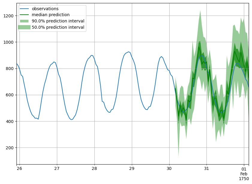
Forecast objects have a plot method that can summarize the forecast paths as the mean, prediction intervals, etc. The prediction intervals are shaded in different colors as a “fan chart”.
[24]:
def plot_prob_forecasts(ts_entry, forecast_entry):
    plot_length = 150
    prediction_intervals = (50.0, 90.0)
    legend = ["observations", "median prediction"] + [
        f"{k}% prediction interval" for k in prediction_intervals
    ][::-1]

    fig, ax = plt.subplots(1, 1, figsize=(10, 7))
    ts_entry[-plot_length:].plot(ax=ax)  # plot the time series
    forecast_entry.plot(prediction_intervals=prediction_intervals, color="g")
    plt.grid(which="both")
    plt.legend(legend, loc="upper left")
    plt.show()
[25]:
plot_prob_forecasts(ts_entry, forecast_entry)
We can also evaluate the quality of our forecasts numerically. In GluonTS, the Evaluator class can compute aggregate performance metrics, as well as metrics per time series (which can be useful for analyzing performance across heterogeneous time series).
[26]:
from gluonts.evaluation import Evaluator
[27]:
evaluator = Evaluator(quantiles=[0.1, 0.5, 0.9])
agg_metrics, item_metrics = evaluator(tss, forecasts)
Running evaluation: 414it [00:00, 17460.80it/s]
The aggregate metrics, agg_metrics, aggregate both across time-steps and across time series.
[28]:
print(json.dumps(agg_metrics, indent=4))
{
    "MSE": 14103503.490942253,
    "abs_error": 11394017.439418793,
    "abs_target_sum": 145558863.59960938,
    "abs_target_mean": 7324.822041043146,
    "seasonal_error": 336.9046924038305,
    "MASE": 4.508370962998624,
    "MAPE": 0.26704551166766316,
    "sMAPE": 0.20000923968455642,
    "MSIS": 64.95399372682238,
    "QuantileLoss[0.1]": 5287861.744539069,
    "Coverage[0.1]": 0.10653180354267312,
    "QuantileLoss[0.5]": 11394017.344079018,
    "Coverage[0.5]": 0.5231481481481481,
    "QuantileLoss[0.9]": 7136587.792640017,
    "Coverage[0.9]": 0.8730877616747181,
    "RMSE": 3755.4631526540443,
    "NRMSE": 0.5127036713808298,
    "ND": 0.0782777301062233,
    "wQuantileLoss[0.1]": 0.036327995518599665,
    "wQuantileLoss[0.5]": 0.0782777294512321,
    "wQuantileLoss[0.9]": 0.0490288781882134,
    "mean_absolute_QuantileLoss": 7939488.960419368,
    "mean_wQuantileLoss": 0.05454486771934839,
    "MAE_Coverage": 0.3910292538915727,
    "OWA": NaN
}
Individual metrics are aggregated only across time-steps.
[29]:
item_metrics.head()
[29]:
| item_id | forecast_start | MSE | abs_error | abs_target_sum | abs_target_mean | seasonal_error | MASE | MAPE | sMAPE | ND | MSIS | QuantileLoss[0.1] | Coverage[0.1] | QuantileLoss[0.5] | Coverage[0.5] | QuantileLoss[0.9] | Coverage[0.9] | |
|---|---|---|---|---|---|---|---|---|---|---|---|---|---|---|---|---|---|---|
| 0 | 0 | 1750-01-30 04:00 | 3935.235352 | 2439.343506 | 31644.0 | 659.250000 | 42.371302 | 1.199389 | 0.077174 | 0.075758 | 0.077087 | 13.375761 | 1005.179742 | 0.020833 | 2439.343536 | 0.708333 | 1450.966931 | 0.979167 |
| 1 | 1 | 1750-01-30 04:00 | 190986.354167 | 17802.804688 | 124149.0 | 2586.437500 | 165.107988 | 2.246359 | 0.146013 | 0.133097 | 0.143399 | 14.318695 | 5224.894556 | 0.250000 | 17802.803711 | 0.916667 | 8510.102588 | 1.000000 |
| 2 | 2 | 1750-01-30 04:00 | 31228.807292 | 6641.527832 | 65030.0 | 1354.791667 | 78.889053 | 1.753921 | 0.095075 | 0.101465 | 0.102130 | 13.730244 | 3504.432349 | 0.000000 | 6641.527954 | 0.145833 | 2398.131860 | 0.833333 |
| 3 | 3 | 1750-01-30 04:00 | 219602.145833 | 17370.642578 | 235783.0 | 4912.145833 | 258.982249 | 1.397348 | 0.073054 | 0.073218 | 0.073672 | 15.614696 | 10792.337207 | 0.020833 | 17370.642578 | 0.375000 | 8332.165234 | 0.937500 |
| 4 | 4 | 1750-01-30 04:00 | 135302.041667 | 13298.474609 | 131088.0 | 2731.000000 | 200.494083 | 1.381844 | 0.101289 | 0.096023 | 0.101447 | 13.013480 | 5403.914014 | 0.062500 | 13298.474609 | 0.666667 | 7285.936548 | 1.000000 |
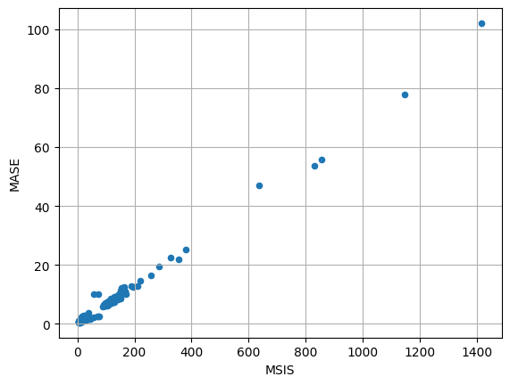
[30]:
item_metrics.plot(x="MSIS", y="MASE", kind="scatter")
plt.grid(which="both")
plt.show()