Quick Start Tutorial#
GluonTS contains:
A number of pre-built models
Components for building new models (likelihoods, feature processing pipelines, calendar features etc.)
Data loading and processing
Plotting and evaluation facilities
Artificial and real datasets (only external datasets with blessed license)
[1]:
# %#matplotlib inline
import mxnet as mx
from mxnet import gluon
import numpy as np
import pandas as pd
import matplotlib.pyplot as plt
import json
Datasets#
Provided datasets#
GluonTS comes with a number of publicly available datasets.
[2]:
from gluonts.dataset.repository.datasets import get_dataset, dataset_recipes
from gluonts.dataset.util import to_pandas
[3]:
print(f"Available datasets: {list(dataset_recipes.keys())}")
Available datasets: ['constant', 'exchange_rate', 'solar-energy', 'electricity', 'traffic', 'exchange_rate_nips', 'electricity_nips', 'traffic_nips', 'solar_nips', 'wiki-rolling_nips', 'taxi_30min', 'kaggle_web_traffic_with_missing', 'kaggle_web_traffic_without_missing', 'kaggle_web_traffic_weekly', 'm1_yearly', 'm1_quarterly', 'm1_monthly', 'nn5_daily_with_missing', 'nn5_daily_without_missing', 'nn5_weekly', 'tourism_monthly', 'tourism_quarterly', 'tourism_yearly', 'cif_2016', 'london_smart_meters_without_missing', 'wind_farms_without_missing', 'car_parts_without_missing', 'dominick', 'fred_md', 'pedestrian_counts', 'hospital', 'covid_deaths', 'kdd_cup_2018_without_missing', 'weather', 'm3_monthly', 'm3_quarterly', 'm3_yearly', 'm3_other', 'm4_hourly', 'm4_daily', 'm4_weekly', 'm4_monthly', 'm4_quarterly', 'm4_yearly', 'm5', 'uber_tlc_daily', 'uber_tlc_hourly', 'airpassengers']
To download one of the built-in datasets, simply call get_dataset with one of the above names. GluonTS can re-use the saved dataset so that it does not need to be downloaded again the next time around.
[4]:
dataset = get_dataset("m4_hourly")
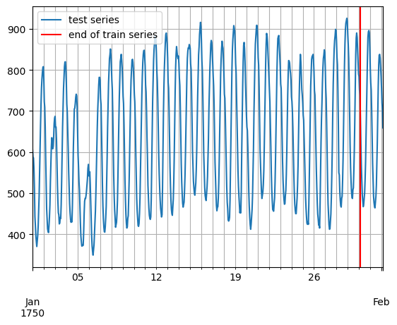
In general, the datasets provided by GluonTS are objects that consists of three main members:
dataset.trainis an iterable collection of data entries used for training. Each entry corresponds to one time series.dataset.testis an iterable collection of data entries used for inference. The test dataset is an extended version of the train dataset that contains a window in the end of each time series that was not seen during training. This window has length equal to the recommended prediction length.dataset.metadatacontains metadata of the dataset such as the frequency of the time series, a recommended prediction horizon, associated features, etc.
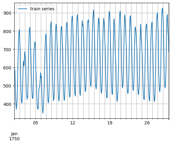
[5]:
entry = next(iter(dataset.train))
train_series = to_pandas(entry)
train_series.plot()
plt.grid(which="both")
plt.legend(["train series"], loc="upper left")
plt.show()
[6]:
entry = next(iter(dataset.test))
test_series = to_pandas(entry)
test_series.plot()
plt.axvline(train_series.index[-1], color="r")  # end of train dataset
plt.grid(which="both")
plt.legend(["test series", "end of train series"], loc="upper left")
plt.show()
[7]:
print(
    f"Length of forecasting window in test dataset: {len(test_series) - len(train_series)}"
)
print(f"Recommended prediction horizon: {dataset.metadata.prediction_length}")
print(f"Frequency of the time series: {dataset.metadata.freq}")
Length of forecasting window in test dataset: 48
Recommended prediction horizon: 48
Frequency of the time series: H
Custom datasets#
At this point, it is important to emphasize that GluonTS does not require this specific format for a custom dataset that a user may have. The only requirements for a custom dataset are to be iterable and have a “target” and a “start” field. To make this more clear, assume the common case where a dataset is in the form of a numpy.array and the index of the time series in a pandas.Period (possibly different for each time series):
[8]:
N = 10  # number of time series
T = 100  # number of timesteps
prediction_length = 24
freq = "1H"
custom_dataset = np.random.normal(size=(N, T))
start = pd.Period("01-01-2019", freq=freq)  # can be different for each time series
Now, you can split your dataset and bring it in a GluonTS appropriate format with just two lines of code:
[9]:
from gluonts.dataset.common import ListDataset
[10]:
# train dataset: cut the last window of length "prediction_length", add "target" and "start" fields
train_ds = ListDataset(
    [{"target": x, "start": start} for x in custom_dataset[:, :-prediction_length]],
    freq=freq,
)
# test dataset: use the whole dataset, add "target" and "start" fields
test_ds = ListDataset(
    [{"target": x, "start": start} for x in custom_dataset], freq=freq
)
Training an existing model (Estimator)#
GluonTS comes with a number of pre-built models. All the user needs to do is configure some hyperparameters. The existing models focus on (but are not limited to) probabilistic forecasting. Probabilistic forecasts are predictions in the form of a probability distribution, rather than simply a single point estimate.
We will begin with GluonTS’s pre-built feedforward neural network estimator, a simple but powerful forecasting model. We will use this model to demonstrate the process of training a model, producing forecasts, and evaluating the results.
GluonTS’s built-in feedforward neural network (SimpleFeedForwardEstimator) accepts an input window of length context_length and predicts the distribution of the values of the subsequent prediction_length values. In GluonTS parlance, the feedforward neural network model is an example of an Estimator. In GluonTS, Estimator objects represent a forecasting model as well as details such as its coefficients, weights, etc.
In general, each estimator (pre-built or custom) is configured by a number of hyperparameters that can be either common (but not binding) among all estimators (e.g., the prediction_length) or specific for the particular estimator (e.g., number of layers for a neural network or the stride in a CNN).
Finally, each estimator is configured by a Trainer, which defines how the model will be trained i.e., the number of epochs, the learning rate, etc.
[11]:
from gluonts.mx import SimpleFeedForwardEstimator, Trainer
[12]:
estimator = SimpleFeedForwardEstimator(
    num_hidden_dimensions=[10],
    prediction_length=dataset.metadata.prediction_length,
    context_length=100,
    trainer=Trainer(ctx="cpu", epochs=5, learning_rate=1e-3, num_batches_per_epoch=100),
)
After specifying our estimator with all the necessary hyperparameters we can train it using our training dataset dataset.train by invoking the train method of the estimator. The training algorithm returns a fitted model (or a Predictor in GluonTS parlance) that can be used to construct forecasts.
[13]:
predictor = estimator.train(dataset.train)
100%|██████████| 100/100 [00:01<00:00, 86.55it/s, epoch=1/5, avg_epoch_loss=5.53]
100%|██████████| 100/100 [00:01<00:00, 85.80it/s, epoch=2/5, avg_epoch_loss=4.84]
100%|██████████| 100/100 [00:01<00:00, 88.24it/s, epoch=3/5, avg_epoch_loss=4.83]
100%|██████████| 100/100 [00:01<00:00, 87.69it/s, epoch=4/5, avg_epoch_loss=4.64]
100%|██████████| 100/100 [00:01<00:00, 88.18it/s, epoch=5/5, avg_epoch_loss=4.75]
Visualize and evaluate forecasts#
With a predictor in hand, we can now predict the last window of the dataset.test and evaluate our model’s performance.
GluonTS comes with the make_evaluation_predictions function that automates the process of prediction and model evaluation. Roughly, this function performs the following steps:
Removes the final window of length
prediction_lengthof thedataset.testthat we want to predictThe estimator uses the remaining data to predict (in the form of sample paths) the “future” window that was just removed
The module outputs the forecast sample paths and the
dataset.test(as python generator objects)
[14]:
from gluonts.evaluation import make_evaluation_predictions
[15]:
forecast_it, ts_it = make_evaluation_predictions(
    dataset=dataset.test,  # test dataset
    predictor=predictor,  # predictor
    num_samples=100,  # number of sample paths we want for evaluation
)
First, we can convert these generators to lists to ease the subsequent computations.
[16]:
forecasts = list(forecast_it)
tss = list(ts_it)
We can examine the first element of these lists (that corresponds to the first time series of the dataset). Let’s start with the list containing the time series, i.e., tss. We expect the first entry of tss to contain the (target of the) first time series of dataset.test.
[17]:
# first entry of the time series list
ts_entry = tss[0]
[18]:
# first 5 values of the time series (convert from pandas to numpy)
np.array(ts_entry[:5]).reshape(
    -1,
)
[18]:
array([605., 586., 586., 559., 511.], dtype=float32)
[19]:
# first entry of dataset.test
dataset_test_entry = next(iter(dataset.test))
[20]:
# first 5 values
dataset_test_entry["target"][:5]
[20]:
array([605., 586., 586., 559., 511.], dtype=float32)
The entries in the forecast list are a bit more complex. They are objects that contain all the sample paths in the form of numpy.ndarray with dimension (num_samples, prediction_length), the start date of the forecast, the frequency of the time series, etc. We can access all this information by simply invoking the corresponding attribute of the forecast object.
[21]:
# first entry of the forecast list
forecast_entry = forecasts[0]
[22]:
print(f"Number of sample paths: {forecast_entry.num_samples}")
print(f"Dimension of samples: {forecast_entry.samples.shape}")
print(f"Start date of the forecast window: {forecast_entry.start_date}")
print(f"Frequency of the time series: {forecast_entry.freq}")
Number of sample paths: 100
Dimension of samples: (100, 48)
Start date of the forecast window: 1750-01-30 04:00
Frequency of the time series: <Hour>
We can also do calculations to summarize the sample paths, such as computing the mean or a quantile for each of the 48 time steps in the forecast window.
[23]:
print(f"Mean of the future window:\n {forecast_entry.mean}")
print(f"0.5-quantile (median) of the future window:\n {forecast_entry.quantile(0.5)}")
Mean of the future window:
 [691.85095 693.6895  465.42505 590.9533  498.43475 447.46643 396.5832
 500.63547 522.3127  577.0875  657.5044  743.4836  658.5824  743.11115
 815.3825  824.47656 902.9747  816.2875  827.56055 834.44995 786.1446
 808.23975 690.2347  646.11127 559.55994 522.6163  579.84344 440.77704
 406.83047 513.3476  476.45844 511.00632 531.5564  563.4689  675.0758
 714.1624  709.24963 823.404   801.76    863.0185  776.3015  825.3122
 844.1778  821.53845 839.9411  767.74603 646.74146 677.1551 ]
0.5-quantile (median) of the future window:
 [703.04913 680.69763 495.85205 594.3352  490.2174  452.98758 412.19336
 504.45535 521.8173  561.7406  656.6593  730.7509  685.08636 750.5102
 814.05115 843.2447  910.45917 829.26965 832.38824 835.2924  803.2559
 792.89355 686.09937 640.87775 557.698   533.8995  581.88696 440.08337
 432.26544 503.29816 472.9545  503.22687 521.0031  557.6608  664.80365
 699.97406 695.20874 825.4764  793.77875 884.8748  779.93866 845.66455
 846.6589  797.7362  822.82275 772.314   656.8639  679.34357]
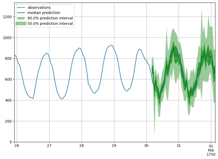
Forecast objects have a plot method that can summarize the forecast paths as the mean, prediction intervals, etc. The prediction intervals are shaded in different colors as a “fan chart”.
[24]:
def plot_prob_forecasts(ts_entry, forecast_entry):
    plot_length = 150
    prediction_intervals = (50.0, 90.0)
    legend = ["observations", "median prediction"] + [
        f"{k}% prediction interval" for k in prediction_intervals
    ][::-1]

    fig, ax = plt.subplots(1, 1, figsize=(10, 7))
    ts_entry[-plot_length:].plot(ax=ax)  # plot the time series
    forecast_entry.plot(prediction_intervals=prediction_intervals, color="g")
    plt.grid(which="both")
    plt.legend(legend, loc="upper left")
    plt.show()
[25]:
plot_prob_forecasts(ts_entry, forecast_entry)
We can also evaluate the quality of our forecasts numerically. In GluonTS, the Evaluator class can compute aggregate performance metrics, as well as metrics per time series (which can be useful for analyzing performance across heterogeneous time series).
[26]:
from gluonts.evaluation import Evaluator
[27]:
evaluator = Evaluator(quantiles=[0.1, 0.5, 0.9])
agg_metrics, item_metrics = evaluator(tss, forecasts)
Running evaluation: 414it [00:00, 15902.79it/s]
The aggregate metrics, agg_metrics, aggregate both across time-steps and across time series.
[28]:
print(json.dumps(agg_metrics, indent=4))
{
    "MSE": 9392223.75122387,
    "abs_error": 9963095.421772003,
    "abs_target_sum": 145558863.59960938,
    "abs_target_mean": 7324.822041043146,
    "seasonal_error": 336.9046924038305,
    "MASE": 4.969079049006028,
    "MAPE": 0.2566654594696086,
    "sMAPE": 0.2064668832289808,
    "MSIS": 66.52445687385355,
    "QuantileLoss[0.1]": 6114005.78946724,
    "Coverage[0.1]": 0.09566223832528181,
    "QuantileLoss[0.5]": 9963095.456448555,
    "Coverage[0.5]": 0.421749194847021,
    "QuantileLoss[0.9]": 6620538.404082298,
    "Coverage[0.9]": 0.8645330112721417,
    "RMSE": 3064.673514621724,
    "NRMSE": 0.4183956275592023,
    "ND": 0.06844719157177276,
    "wQuantileLoss[0.1]": 0.04200366530948684,
    "wQuantileLoss[0.5]": 0.0684471918100032,
    "wQuantileLoss[0.9]": 0.04548358128360701,
    "mean_absolute_QuantileLoss": 7565879.883332697,
    "mean_wQuantileLoss": 0.05197814613436569,
    "MAE_Coverage": 0.03935185185185185,
    "OWA": NaN
}
Individual metrics are aggregated only across time-steps.
[29]:
item_metrics.head()
[29]:
| item_id | forecast_start | MSE | abs_error | abs_target_sum | abs_target_mean | seasonal_error | MASE | MAPE | sMAPE | ND | MSIS | QuantileLoss[0.1] | Coverage[0.1] | QuantileLoss[0.5] | Coverage[0.5] | QuantileLoss[0.9] | Coverage[0.9] | |
|---|---|---|---|---|---|---|---|---|---|---|---|---|---|---|---|---|---|---|
| 0 | 0 | 1750-01-30 04:00 | 3278.552734 | 2088.441650 | 31644.0 | 659.250000 | 42.371302 | 1.026855 | 0.069766 | 0.068469 | 0.065998 | 14.859941 | 1280.970441 | 0.062500 | 2088.441681 | 0.583333 | 1363.438116 | 1.000000 |
| 1 | 1 | 1750-01-30 04:00 | 135613.500000 | 14760.962891 | 124149.0 | 2586.437500 | 165.107988 | 1.862539 | 0.129558 | 0.117889 | 0.118897 | 14.320504 | 5198.448267 | 0.229167 | 14760.962402 | 0.895833 | 8079.475879 | 1.000000 |
| 2 | 2 | 1750-01-30 04:00 | 56107.635417 | 8608.524414 | 65030.0 | 1354.791667 | 78.889053 | 2.273373 | 0.119546 | 0.130265 | 0.132378 | 14.682484 | 3960.515662 | 0.000000 | 8608.524170 | 0.229167 | 3968.368433 | 0.687500 |
| 3 | 3 | 1750-01-30 04:00 | 318093.666667 | 22859.949219 | 235783.0 | 4912.145833 | 258.982249 | 1.838925 | 0.093685 | 0.096479 | 0.096953 | 15.911051 | 11323.955127 | 0.041667 | 22859.950928 | 0.375000 | 8394.896484 | 0.895833 |
| 4 | 4 | 1750-01-30 04:00 | 64661.864583 | 9039.398438 | 131088.0 | 2731.000000 | 200.494083 | 0.939284 | 0.071480 | 0.069498 | 0.068957 | 13.737920 | 5459.190002 | 0.000000 | 9039.398193 | 0.645833 | 6914.293408 | 1.000000 |
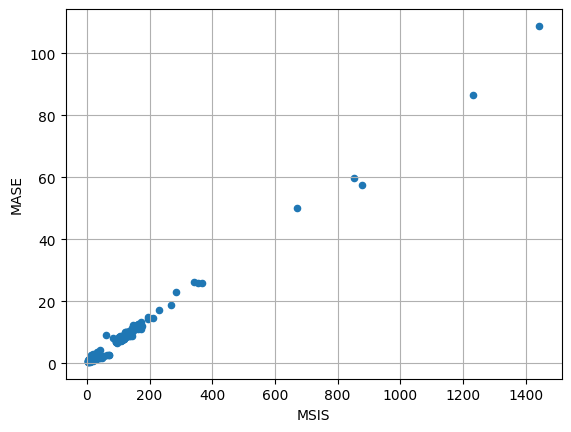
[30]:
item_metrics.plot(x="MSIS", y="MASE", kind="scatter")
plt.grid(which="both")
plt.show()