Quick Start Tutorial#
GluonTS contains:
A number of pre-built models
Components for building new models (likelihoods, feature processing pipelines, calendar features etc.)
Data loading and processing
Plotting and evaluation facilities
Artificial and real datasets (only external datasets with blessed license)
[1]:
%matplotlib inline
import numpy as np
import pandas as pd
import matplotlib.pyplot as plt
import json
Datasets#
Provided datasets#
GluonTS comes with a number of publicly available datasets.
[2]:
from gluonts.dataset.repository import get_dataset, dataset_names
from gluonts.dataset.util import to_pandas
[3]:
print(f"Available datasets: {dataset_names}")
Available datasets: ['constant', 'exchange_rate', 'solar-energy', 'electricity', 'traffic', 'exchange_rate_nips', 'electricity_nips', 'traffic_nips', 'solar_nips', 'wiki2000_nips', 'wiki-rolling_nips', 'taxi_30min', 'kaggle_web_traffic_with_missing', 'kaggle_web_traffic_without_missing', 'kaggle_web_traffic_weekly', 'm1_yearly', 'm1_quarterly', 'm1_monthly', 'nn5_daily_with_missing', 'nn5_daily_without_missing', 'nn5_weekly', 'tourism_monthly', 'tourism_quarterly', 'tourism_yearly', 'cif_2016', 'london_smart_meters_without_missing', 'wind_farms_without_missing', 'car_parts_without_missing', 'dominick', 'fred_md', 'pedestrian_counts', 'hospital', 'covid_deaths', 'kdd_cup_2018_without_missing', 'weather', 'm3_monthly', 'm3_quarterly', 'm3_yearly', 'm3_other', 'm4_hourly', 'm4_daily', 'm4_weekly', 'm4_monthly', 'm4_quarterly', 'm4_yearly', 'm5', 'uber_tlc_daily', 'uber_tlc_hourly', 'airpassengers', 'australian_electricity_demand', 'electricity_hourly', 'electricity_weekly', 'rideshare_without_missing', 'saugeenday', 'solar_10_minutes', 'solar_weekly', 'sunspot_without_missing', 'temperature_rain_without_missing', 'vehicle_trips_without_missing', 'ercot', 'ett_small_15min', 'ett_small_1h']
To download one of the built-in datasets, simply call get_dataset with one of the above names. GluonTS can re-use the saved dataset so that it does not need to be downloaded again the next time around.
[4]:
dataset = get_dataset("m4_hourly")
In general, the datasets provided by GluonTS are objects that consists of three main members:
dataset.trainis an iterable collection of data entries used for training. Each entry corresponds to one time series.dataset.testis an iterable collection of data entries used for inference. The test dataset is an extended version of the train dataset that contains a window in the end of each time series that was not seen during training. This window has length equal to the recommended prediction length.dataset.metadatacontains metadata of the dataset such as the frequency of the time series, a recommended prediction horizon, associated features, etc.
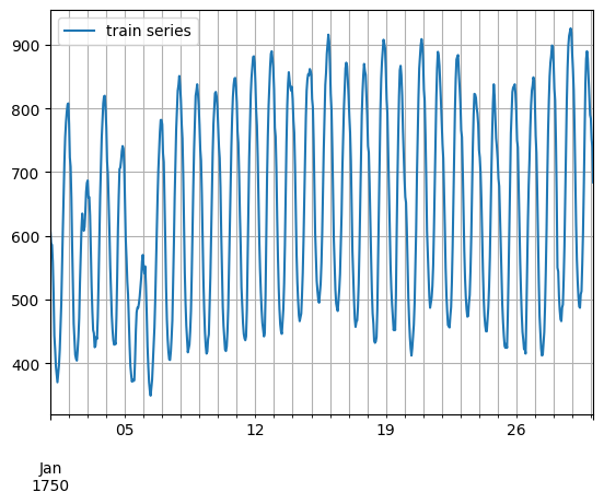
[5]:
entry = next(iter(dataset.train))
train_series = to_pandas(entry)
train_series.plot()
plt.grid(which="both")
plt.legend(["train series"], loc="upper left")
plt.show()
/opt/hostedtoolcache/Python/3.11.15/x64/lib/python3.11/site-packages/gluonts/dataset/common.py:263: FutureWarning: 'H' is deprecated and will be removed in a future version, please use 'h' instead.
  return pd.Period(val, freq)
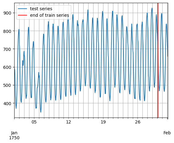
[6]:
entry = next(iter(dataset.test))
test_series = to_pandas(entry)
test_series.plot()
plt.axvline(train_series.index[-1], color="r")  # end of train dataset
plt.grid(which="both")
plt.legend(["test series", "end of train series"], loc="upper left")
plt.show()
[7]:
print(
    f"Length of forecasting window in test dataset: {len(test_series) - len(train_series)}"
)
print(f"Recommended prediction horizon: {dataset.metadata.prediction_length}")
print(f"Frequency of the time series: {dataset.metadata.freq}")
Length of forecasting window in test dataset: 48
Recommended prediction horizon: 48
Frequency of the time series: H
Custom datasets#
At this point, it is important to emphasize that GluonTS does not require this specific format for a custom dataset that a user may have. The only requirements for a custom dataset are to be iterable and have a “target” and a “start” field. To make this more clear, assume the common case where a dataset is in the form of a numpy.array and the index of the time series in a pandas.Period (possibly different for each time series):
[8]:
N = 10  # number of time series
T = 100  # number of timesteps
prediction_length = 24
freq = "1H"
custom_dataset = np.random.normal(size=(N, T))
start = pd.Period("01-01-2019", freq=freq)  # can be different for each time series
/tmp/ipykernel_3646/2007592095.py:6: FutureWarning: 'H' is deprecated and will be removed in a future version, please use 'h' instead.
  start = pd.Period("01-01-2019", freq=freq)  # can be different for each time series
Now, you can split your dataset and bring it in a GluonTS appropriate format with just two lines of code:
[9]:
from gluonts.dataset.common import ListDataset
[10]:
# train dataset: cut the last window of length "prediction_length", add "target" and "start" fields
train_ds = ListDataset(
    [{"target": x, "start": start} for x in custom_dataset[:, :-prediction_length]],
    freq=freq,
)
# test dataset: use the whole dataset, add "target" and "start" fields
test_ds = ListDataset(
    [{"target": x, "start": start} for x in custom_dataset], freq=freq
)
/opt/hostedtoolcache/Python/3.11.15/x64/lib/python3.11/site-packages/gluonts/dataset/common.py:255: FutureWarning: 'H' is deprecated and will be removed in a future version, please use 'h' instead.
  ProcessDataEntry(to_offset(freq), one_dim_target, use_timestamp),
Training an existing model (Estimator)#
GluonTS comes with a number of pre-built models. All the user needs to do is configure some hyperparameters. The existing models focus on (but are not limited to) probabilistic forecasting. Probabilistic forecasts are predictions in the form of a probability distribution, rather than simply a single point estimate.
We will begin with GluonTS’s pre-built feedforward neural network estimator, a simple but powerful forecasting model. We will use this model to demonstrate the process of training a model, producing forecasts, and evaluating the results.
GluonTS’s built-in feedforward neural network (SimpleFeedForwardEstimator) accepts an input window of length context_length and predicts the distribution of the values of the subsequent prediction_length values. In GluonTS parlance, the feedforward neural network model is an example of an Estimator. In GluonTS, Estimator objects represent a forecasting model as well as details such as its coefficients, weights, etc.
In general, each estimator (pre-built or custom) is configured by a number of hyperparameters that can be either common (but not binding) among all estimators (e.g., the prediction_length) or specific for the particular estimator (e.g., number of layers for a neural network or the stride in a CNN).
Finally, each estimator is configured by a Trainer, which defines how the model will be trained i.e., the number of epochs, the learning rate, etc.
[11]:
from gluonts.mx import SimpleFeedForwardEstimator, Trainer
[12]:
estimator = SimpleFeedForwardEstimator(
    num_hidden_dimensions=[10],
    prediction_length=dataset.metadata.prediction_length,
    context_length=100,
    trainer=Trainer(ctx="cpu", epochs=5, learning_rate=1e-3, num_batches_per_epoch=100),
)
After specifying our estimator with all the necessary hyperparameters we can train it using our training dataset dataset.train by invoking the train method of the estimator. The training algorithm returns a fitted model (or a Predictor in GluonTS parlance) that can be used to construct forecasts.
[13]:
predictor = estimator.train(dataset.train)
100%|██████████| 100/100 [00:00<00:00, 162.18it/s, epoch=1/5, avg_epoch_loss=5.48]
100%|██████████| 100/100 [00:00<00:00, 172.34it/s, epoch=2/5, avg_epoch_loss=4.79]
100%|██████████| 100/100 [00:00<00:00, 164.59it/s, epoch=3/5, avg_epoch_loss=4.83]
100%|██████████| 100/100 [00:00<00:00, 171.07it/s, epoch=4/5, avg_epoch_loss=4.77]
100%|██████████| 100/100 [00:00<00:00, 166.74it/s, epoch=5/5, avg_epoch_loss=4.79]
Visualize and evaluate forecasts#
With a predictor in hand, we can now predict the last window of the dataset.test and evaluate our model’s performance.
GluonTS comes with the make_evaluation_predictions function that automates the process of prediction and model evaluation. Roughly, this function performs the following steps:
Removes the final window of length
prediction_lengthof thedataset.testthat we want to predictThe estimator uses the remaining data to predict (in the form of sample paths) the “future” window that was just removed
The module outputs the forecast sample paths and the
dataset.test(as python generator objects)
[14]:
from gluonts.evaluation import make_evaluation_predictions
[15]:
forecast_it, ts_it = make_evaluation_predictions(
    dataset=dataset.test,  # test dataset
    predictor=predictor,  # predictor
    num_samples=100,  # number of sample paths we want for evaluation
)
First, we can convert these generators to lists to ease the subsequent computations.
[16]:
forecasts = list(forecast_it)
tss = list(ts_it)
We can examine the first element of these lists (that corresponds to the first time series of the dataset). Let’s start with the list containing the time series, i.e., tss. We expect the first entry of tss to contain the (target of the) first time series of dataset.test.
[17]:
# first entry of the time series list
ts_entry = tss[0]
[18]:
# first 5 values of the time series (convert from pandas to numpy)
np.array(ts_entry[:5]).reshape(
    -1,
)
[18]:
array([605., 586., 586., 559., 511.], dtype=float32)
[19]:
# first entry of dataset.test
dataset_test_entry = next(iter(dataset.test))
[20]:
# first 5 values
dataset_test_entry["target"][:5]
[20]:
array([605., 586., 586., 559., 511.], dtype=float32)
The entries in the forecast list are a bit more complex. They are objects that contain all the sample paths in the form of numpy.ndarray with dimension (num_samples, prediction_length), the start date of the forecast, the frequency of the time series, etc. We can access all this information by simply invoking the corresponding attribute of the forecast object.
[21]:
# first entry of the forecast list
forecast_entry = forecasts[0]
[22]:
print(f"Number of sample paths: {forecast_entry.num_samples}")
print(f"Dimension of samples: {forecast_entry.samples.shape}")
print(f"Start date of the forecast window: {forecast_entry.start_date}")
print(f"Frequency of the time series: {forecast_entry.freq}")
Number of sample paths: 100
Dimension of samples: (100, 48)
Start date of the forecast window: 1750-01-30 04:00
Frequency of the time series: <Hour>
We can also do calculations to summarize the sample paths, such as computing the mean or a quantile for each of the 48 time steps in the forecast window.
[23]:
print(f"Mean of the future window:\n {forecast_entry.mean}")
print(f"0.5-quantile (median) of the future window:\n {forecast_entry.quantile(0.5)}")
Mean of the future window:
 [619.2102  604.5326  501.43384 531.49805 448.83417 513.5555  498.87503
 507.93195 527.95074 567.98126 615.2731  688.1492  763.5412  799.7254
 924.026   776.8998  804.5237  777.3353  938.16187 865.23346 860.28784
 812.3482  818.84827 627.9241  679.5098  571.81854 584.7185  501.18427
 495.6643  459.60144 457.2102  429.15454 562.30426 549.9289  614.4246
 700.9545  753.2977  943.5215  956.6022  821.2316  899.45825 866.2595
 912.8778  932.13306 852.22327 779.1448  665.4927  741.40466]
0.5-quantile (median) of the future window:
 [633.4381  593.48584 520.0153  533.17975 438.18274 524.0443  506.6019
 506.84656 530.2531  549.66315 614.05365 688.207   786.22565 813.3204
 925.15594 780.4338  827.0789  782.8089  946.8017  844.16864 872.674
 792.2093  811.9395  615.58673 674.28076 578.21466 586.3576  501.6862
 502.55945 466.89633 433.16364 430.452   554.93835 552.09393 607.2102
 688.2682  734.33264 945.7514  942.2568  849.2787  873.6543  881.9464
 918.5369  907.9371  832.8961  781.7563  679.8267  756.3833 ]
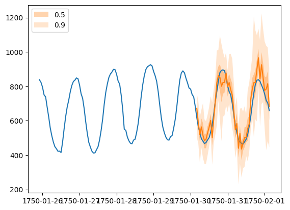
Forecast objects have a plot method that can summarize the forecast paths as the mean, prediction intervals, etc. The prediction intervals are shaded in different colors as a “fan chart”.
[24]:
plt.plot(ts_entry[-150:].to_timestamp())
forecast_entry.plot(show_label=True)
plt.legend()
[24]:
<matplotlib.legend.Legend at 0x7fde684b9890>
We can also evaluate the quality of our forecasts numerically. In GluonTS, the Evaluator class can compute aggregate performance metrics, as well as metrics per time series (which can be useful for analyzing performance across heterogeneous time series).
[25]:
from gluonts.evaluation import Evaluator
[26]:
evaluator = Evaluator(quantiles=[0.1, 0.5, 0.9])
agg_metrics, item_metrics = evaluator(tss, forecasts)
Running evaluation: 414it [00:00, 10073.80it/s]
The aggregate metrics, agg_metrics, aggregate both across time-steps and across time series.
[27]:
print(json.dumps(agg_metrics, indent=4))
{
    "MSE": 13983474.511642246,
    "abs_error": 11055211.876312256,
    "abs_target_sum": 145558863.59960938,
    "abs_target_mean": 7324.822041043146,
    "seasonal_error": 336.9046924038305,
    "MASE": 4.0914133966422765,
    "MAPE": 0.2607057271780215,
    "sMAPE": 0.19400012260977773,
    "MSIS": 67.88261136636154,
    "num_masked_target_values": 0.0,
    "QuantileLoss[0.1]": 5244202.2531312,
    "Coverage[0.1]": 0.09566223832528181,
    "QuantileLoss[0.5]": 11055211.800452232,
    "Coverage[0.5]": 0.5462962962962962,
    "QuantileLoss[0.9]": 7771461.533032797,
    "Coverage[0.9]": 0.8865237520128824,
    "RMSE": 3739.4484234499405,
    "NRMSE": 0.5105173071095386,
    "ND": 0.07595011119846311,
    "wQuantileLoss[0.1]": 0.036028051631101586,
    "wQuantileLoss[0.5]": 0.07595011067729922,
    "wQuantileLoss[0.9]": 0.05339050704881742,
    "mean_absolute_QuantileLoss": 8023625.195538743,
    "mean_wQuantileLoss": 0.055122889785739405,
    "MAE_Coverage": 0.39550791733762747,
    "OWA": NaN
}
Individual metrics are aggregated only across time-steps.
[28]:
item_metrics.head()
[28]:
| item_id | forecast_start | MSE | abs_error | abs_target_sum | abs_target_mean | seasonal_error | MASE | MAPE | sMAPE | num_masked_target_values | ND | MSIS | QuantileLoss[0.1] | Coverage[0.1] | QuantileLoss[0.5] | Coverage[0.5] | QuantileLoss[0.9] | Coverage[0.9] | |
|---|---|---|---|---|---|---|---|---|---|---|---|---|---|---|---|---|---|---|---|
| 0 | 0 | 1750-01-30 04:00 | 4470.365885 | 2533.825195 | 31644.0 | 659.250000 | 42.371302 | 1.245844 | 0.077628 | 0.075288 | 0.0 | 0.080073 | 14.771664 | 1072.615613 | 0.020833 | 2533.825378 | 0.770833 | 1623.322363 | 1.000000 |
| 1 | 1 | 1750-01-30 04:00 | 203226.687500 | 18725.628906 | 124149.0 | 2586.437500 | 165.107988 | 2.362801 | 0.156377 | 0.142288 | 0.0 | 0.150832 | 15.478660 | 4498.722046 | 0.291667 | 18725.630371 | 0.958333 | 9260.768115 | 1.000000 |
| 2 | 2 | 1750-01-30 04:00 | 32237.484375 | 6513.241211 | 65030.0 | 1354.791667 | 78.889053 | 1.720043 | 0.090565 | 0.096580 | 0.0 | 0.100157 | 14.761765 | 3576.135974 | 0.000000 | 6513.241211 | 0.250000 | 2306.350562 | 0.875000 |
| 3 | 3 | 1750-01-30 04:00 | 165572.895833 | 16193.964844 | 235783.0 | 4912.145833 | 258.982249 | 1.302693 | 0.068414 | 0.068845 | 0.0 | 0.068682 | 16.559921 | 9689.840967 | 0.000000 | 16193.964844 | 0.500000 | 8927.450586 | 0.958333 |
| 4 | 4 | 1750-01-30 04:00 | 111217.281250 | 11787.074219 | 131088.0 | 2731.000000 | 200.494083 | 1.224794 | 0.087956 | 0.082756 | 0.0 | 0.089917 | 14.915087 | 4633.427832 | 0.020833 | 11787.074951 | 0.729167 | 8092.443799 | 1.000000 |
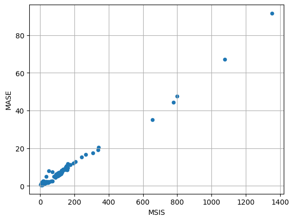
[29]:
item_metrics.plot(x="MSIS", y="MASE", kind="scatter")
plt.grid(which="both")
plt.show()